AP Syllabus focus:
‘Distinguish between uniform and nonuniform partitions of an interval, and compute Riemann sum approximations for both types of partitions.’
This section introduces how dividing an interval into uniform or nonuniform partitions affects the structure of a Riemann sum and how each choice supports approximating definite integrals in practical contexts.
Understanding Interval Partitions
A partition divides an interval [a,b][a, b][a,b] on the xxx-axis into smaller subintervals that allow us to approximate accumulated change using Riemann sums. Because Riemann sums rely on approximating the area under a function with rectangles, understanding how the interval is divided is essential for interpreting the quality and meaning of these approximations in applied problems.
Partition of an interval: A finite set of points dividing [a,b][a, b][a,b] into subintervals whose lengths may be equal or unequal.
When approaching accumulation questions, students must be able to recognize whether a graph, a table of values, or a described scenario is using equally spaced subdivisions or variable-width intervals. This distinction determines how the widths of rectangles are computed and how each sum is constructed.
Uniform Partitions
A uniform partition divides an interval into subintervals of equal width. This structure is particularly common in AP Calculus AB because many tables and diagrams use evenly spaced inputs to simplify Riemann sums.
Uniform partition: A division of [a,b][a, b][a,b] into subintervals where each has the same length Δx\Delta xΔx.
To apply a uniform partition, begin by determining the width of each subinterval. This width is identical across the entire interval and remains constant throughout the sum.
In a uniform partition, every subinterval has the same width, so the partition divides the interval into equal pieces from a to b.

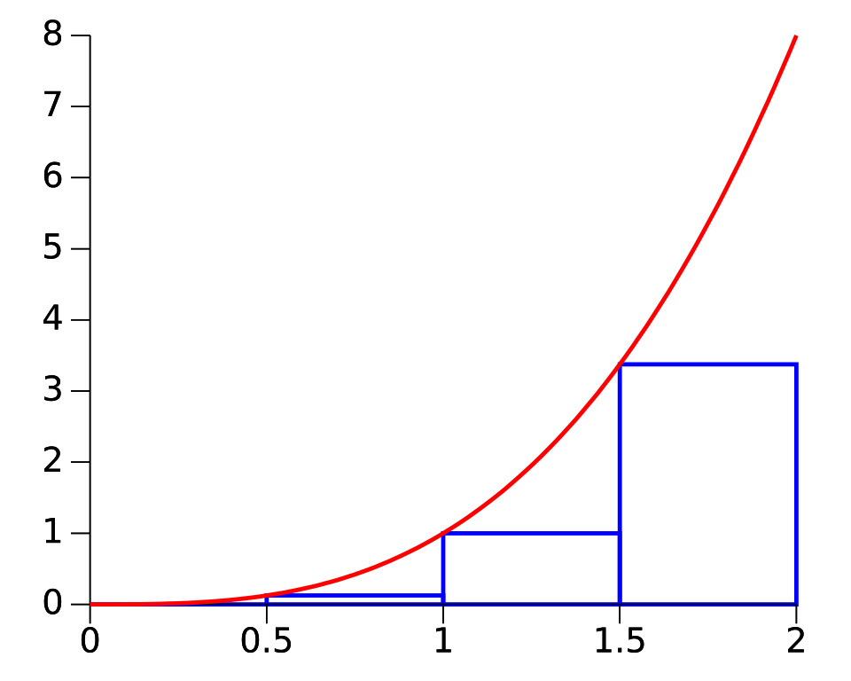
Left Riemann sum on a uniform partition of [0,2][0,2][0,2]. The subintervals all share the same width, and rectangle heights are determined by left-endpoint values. This illustrates how uniform spacing produces equally sized partitions that approximate area under a curve. Source.
= width of each subinterval (units of xxx)
= number of subintervals
= interval endpoints
Uniform partitions support several convenient features useful for AP-level analysis:
They allow predictable placement of left, right, or midpoint sample points.
They produce consistent subinterval widths that streamline symbolic expressions and summation notation.
They make it easy to compare approximation methods on the same interval.
Since uniform spacing simplifies calculations, many textbook approximations and exam-style contexts adopt it. However, real-world data frequently requires a more flexible approach.
Nonuniform Partitions
A nonuniform partition divides the interval into subintervals of differing lengths, determined either by the context or by the available data. Nonuniform spacing occurs naturally in problems where measurements are not collected at equal time intervals or where the geometry of the situation suggests irregular divisions.
Nonuniform partition: A division of [a,b][a, b][a,b] into subintervals whose widths vary and must be computed individually.
Because the subinterval widths differ, each rectangle in the Riemann sum requires separate evaluation, and the width of each must be carefully identified or computed from provided information. In such cases, the Riemann sum is constructed using the specific endpoint values relevant to each subinterval.
In a nonuniform partition, the subinterval widths can differ, so we write them as Δx₁, Δx₂, …, Δxₙ to emphasize that each length may be different.

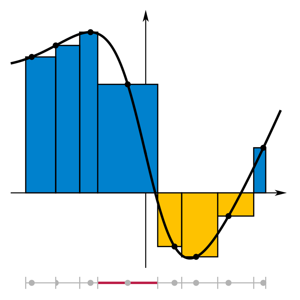
Riemann sum constructed using a nonuniform partition. Each subinterval has a distinct width, and the largest one is highlighted to show variation across the interval. The figure includes an integral expression not required by AP Calculus AB but reinforces how variable-width partitions still produce valid approximations. Source.
A normal sentence is required here before listing structured information, so students are reminded that nonuniform partitions demand precision in identifying interval boundaries before constructing any approximation.
Key elements of nonuniform partitions include:
Subinterval widths Δxi\Delta x_iΔxi change from one subinterval to the next.
Sample points may be chosen in different ways, but each rectangle uses the distinct width of its own subinterval.
Intervals are typically determined directly from a table, graph, or contextual timeline.
Constructing Riemann Sums with Uniform and Nonuniform Partitions
The AP syllabus requires students to compute Riemann sum approximations for both partition types. A Riemann sum is always built from the same conceptual components, but the details depend on how the interval is divided.
Riemann sum: An expression approximating a definite integral by summing products of a function value and a subinterval width.
After the definition, it is important to connect this idea back to the structure of partitions so students understand how these approximations operate across different contexts.
To construct a Riemann sum, use the following layered structure:
Identify the partition points dividing [a,b][a, b][a,b].
Determine whether the partition is uniform (constant Δx\Delta xΔx) or nonuniform (variable Δxi\Delta x_iΔxi).
Choose sample points:
For left sums, use left endpoints.
For right sums, use right endpoints.
For midpoint sums, use the midpoint of each subinterval.
Multiply each function value by the width of its corresponding subinterval.
Add all resulting products to approximate the accumulated area.
How Partitions Affect Accuracy and Interpretation
While the syllabus focus is on distinguishing and computing sums, understanding why the choice of partition matters enhances conceptual clarity. Uniform partitions create consistent rectangles, making patterns easier to analyze, but they may not align with real data. Nonuniform partitions match naturally measured intervals but require careful attention to changing widths.
Because both styles can appear on AP assessments, students must develop fluency recognizing partition types from:
Axis markings on a graph,
Irregular inputs in a table of values,
Descriptions of unevenly spaced measurements in applied scenarios.
Mastering both approaches ensures accurate interpretation of numerical approximations throughout the study of accumulation and integration.
FAQ
A partition is useful when its structure matches the information available about the function. If data points are evenly spaced, a uniform partition maximises efficiency.
When measurements occur at irregular intervals, a non-uniform partition preserves the original spacing, ensuring the approximation remains faithful to the context.
Accuracy depends more on the number and placement of sample points than on uniformity, but partition type still matters.
Uniform partitions often simplify comparison across methods, while non-uniform partitions may capture behaviour more precisely when the function changes rapidly in certain regions.
Real data rarely arrive at equal intervals: sensors record unevenly, time stamps vary, and events can cluster.
Using a non-uniform partition avoids introducing artificial spacing and keeps the approximation consistent with how the data were collected.
Yes. Some problems use partitions where only certain sections have equal widths.
In Riemann sums, each subinterval is treated independently. You compute the width for each interval, regardless of whether neighbouring subintervals match.
Check the horizontal spacing between marked x-values or gridlines beneath the rectangles.
If the base widths of drawn rectangles vary or the x-coordinates of sample points are irregular, the partition is non-uniform.
Practice Questions
A function f is defined on the interval [0, 4]. The partition P = {0, 1, 2, 3, 4} is used to approximate the area under f.
(a) State whether this is a uniform or non-uniform partition.
(b) Give the common width of the subintervals, if it exists.
(1–3 marks)
Question 1 (1–3 marks)
(a) 1 mark
• Uniform partition identified correctly: it is uniform.
(b) 1–2 marks
• 1 mark for stating the common width exists.
• 1 mark for correct width: 1.
A function g is defined and continuous on the interval [2, 10]. A student constructs a Riemann sum using sample points at the right endpoints of each subinterval. The interval is partitioned using P = {2, 3, 5, 6, 9, 10}.
(a) Determine whether the partition is uniform or non-uniform.
(b) Write the widths of all subintervals.
(c) Write the general form of the Riemann sum approximation using the right-endpoint sample points.
(d) Explain how the non-uniformity of the partition affects the interpretation of the Riemann sum.
(4–6 marks)
Question 2 (4–6 marks)
(a) 1 mark
• Correctly identifies the partition as non-uniform.
(b) 1–2 marks
• 1 mark for recognising widths must be calculated individually.
• 1 mark for correctly listing widths: 1, 2, 1, 3, 1.
(c) 1–2 marks
• 1 mark for expressing that each term is g(right endpoint) multiplied by the corresponding subinterval width.
• 1 mark for correctly writing the sum in full:
g(3)(1) + g(5)(2) + g(6)(1) + g(9)(3) + g(10)(1).
(d) 1 mark
• Explains that because the subinterval widths are not equal, each product must use its own width, and the rectangles in the sum vary in size, affecting how the approximation represents the accumulated area.

